Benchmark: ElasticDL Calling Fault-Tolerant AllReduce from Elastic Horovod
In distributed deep learning, the synchronous distributed SGD algorithm works well with dense models used in multimedia applications like speech recognition, image classification, and face recognition. Its asynchronous counterpart works with sparse models with large embeddings for applications like searching, recommending, and advertising.
In a previous benchmark, we tested the performance of ElasticDL working in the asynchronous mode. This one is about synchronous SGD. Like in the previous benchmark, we run three experiments to show that in various cases, ElasticDL can improve the following objectives:
- higher cluster utilization,
- shorter total run time of multiple training jobs, and
- the shorter pending time and higher user satisfaction.
The Dependency on Elastic Horovod
To enable elastic scheduling of synchronous distributed SGD training jobs, we need a fault-tolerable AllReduce. The requirement on fault-tolerance prohibits classical implementations of AllReduce provided by MPI. After a survey, we chose the one from Elastic Horovod released in v0.20.0.
In all the following experiments, the master process of each ElasticDL job calls Kubernetes API to start worker processes, which in turn calls the fault-tolerable AllReduce during distributed training. If jobs with higher-priorities preempt some workers, the master gets notifications and instructs the rest workers to redo the AllReduce. The fault-tolerance feature of the AllReduce implementation prevents all workers from crashing due to the preemption and gives the master the chance to reorganize the rest living workers to make a new AllReduce call.
Experiment Settings
We run experiments on GPU clusters managed by Alibaba Cloud Container Service for Kubernetes (ACK), which features a customized version of Kubernetes. ElasticDL users should be able to repeat all experiments on any modern Kubernetes version that supports priority-aware scheduling.
All experiments use the CIFAR-10 dataset to train a ResNet20 model, a classical image classification model.
Experiment 1: Elastic Scheduling of Multiple ElasticDL Jobs
Consider that two training jobs request more GPUs than what we have in the cluster. Without elastic scheduling, we would have to run them one after another. The submitter of the second job would have to wait for the completion of the first one. The waiting implies a long pending time and bad user experience. It also lowers the GPU utilization and the profit margin of the cloud service.
With elastic scheduling, both jobs run in parallel; each uses less number of GPUs than requested. This approach fully uses all GPUs, shortens the pending time as well as the total running time.
The following figure compares the gang (non-elastic) and elastic scheduling using ElasticDL. The Kubernetes cluster has 6 GPUs, and each of the two jobs requests 4 GPUs.
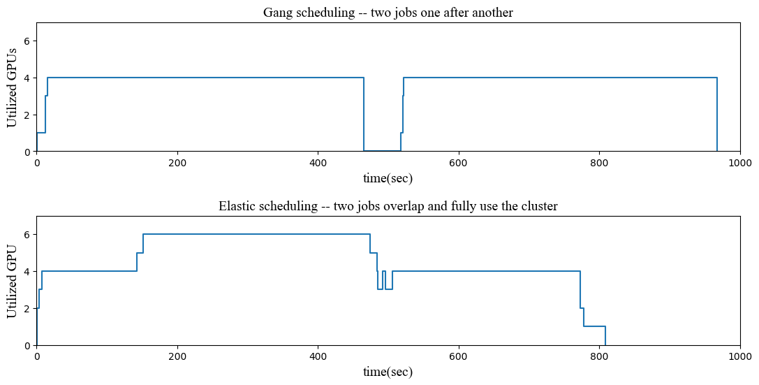
The upper part of the figure presents the GPU utilization over time without elastic scheduling. We see that the two jobs run one after another. Between them, there was a short period of resource allocation by Kubernetes for the second job. The second job ended at 968s. In most of the period, only 4 of the 6 GPUs are in use, and the utilization is as low as 66.6%.
The lower part shows elastic scheduling by ElasticDL enables parallel execution of the two jobs, one using 4 GPUs and another using 2 GPUs – less than the requested 4. We submitted the second job slightly after the first one at 120s. The parallel execution fully utilizes all 6 GPUs until the completion of the first job at 474s. After then, the second job scales up to use 4 GPUs and ends at 809s. The cluster’s overall utilization is higher, and the total run time is less (809s v.s. 968s). Most importantly, users enjoy that both jobs started running once after their submissions.
Experiment 2: Hybrid Deployment of Training Jobs and Serving Service
Many Internet products rely on deep learning inference services. Like any online service, the cluster must keep some extra idle resources to handle unexpected traffic boost, for example, Black Friday.
To use the idle resource, we can run ElasticDL training jobs with lower priorities than the inference service. To verify the idea, we run the following experiment.
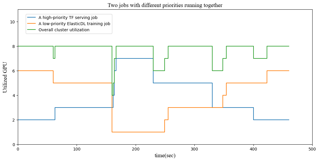
This experiment uses a Kubernetes cluster with 8 GPUs. We start a TensorFlow Serving service and an ElasticDL training job — a script program mimics user traffic to the service.
Initially, the TF serving uses 2 GPUs, and the training job uses 2. In the first 170s, the traffic increase, and Kubernetes’s horizontal scaling feature will increase service processes which will preempt the processes of training jobs. So We can see the auto-increment of service processes and the decrement of training workers.
Then, the script program mimics the decrease of traffic. Kubernetes frees up service processes from using 6 GPUs to 2, as shown by the blue curve. The master process of the ElasticDL job notices this change and increases the number of workers to make use of the freed-up GPUs, as shown in the brown curve.
Anyway, GPUs’ overall utilization is 100% except for short periods when Kubernetes or ElasticDL master was reacting to the change of traffic, as shown by the green curve. The full utilization of GPUs improves the margin profit of cloud service.
Experiment 3: Convergence Tolerant to the Varying Number of Workers
Some users might worry about the convergence as the number of workers might change, which changes the effective batch size. In a vast number of experiments, we observed that, as long as we use the commonly-used trick of learning rate decay, the convergence has no difference between the gang and elastic scheduling.
The following figure shows several experiments training the ResNet20 model with the CIFAR10 dataset. Each worker uses an NVIDIA Tesla P100 GPU. Curves marked “baseline” corresponds to experiments using gang scheduling, and the mark “elastic” denotes ElasticDL jobs.
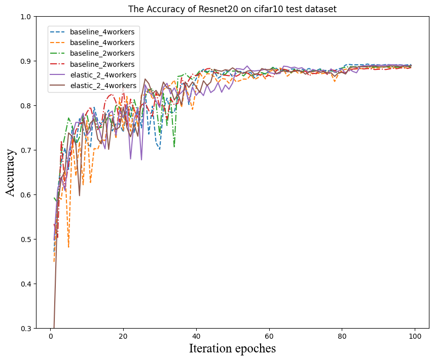
ElasticDL allows users to define a function of learning rate decay. This experiment uses the following decay function.
def callbacks():
    def _schedule(epoch):
        LR = 0.001
        if epoch > 80:
            lr = LR * 0.01
        elif epoch > 60:
            lr = LR * 0.1
        elif epoch > 40:
            lr = LR * 0.5
        else:
            lr = LR
        return lr * hvd.size()

    return [LearningRateScheduler(_schedule)]